

| GEATbx: | Main page Tutorial Algorithms M-functions Parameter/Options Example functions www.geatbx.com |
The population models may be distinguished from each other by looking at the range of the selection strategies of the parents and the definition of the selection pool. Three population models can be defined:
Figure 8-1 presents the corresponding selection pool.
Fig. 8-1: Classification of population models by range of selection (selection pool)
8.1 Global model - worker/farmer |
The global model does not divide the population. Instead, the global model employs the inherent parallelism of evolutionary algorithms (population of individuals). The global model corresponds to the classical evolutionary algorithm.
The calculations where the whole population is needed - fitness assignment and selection - are performed by the master. All remaining calculations which are performed for one or two individuals each can be distributed to a number of slaves. The slaves perform recombination, mutation and the evaluation of the objective function separately. This is known as synchronous master-slave-structure, see figure 8-2.
Fig. 8-2: Global population model (master-slave-structure)
The slave calculations can be done in parallel. For most problems the evaluation of the objective function is the most time consuming part. In this case, the whole evolutionary algorithm is calculated by the master and only the objective function evaluation is distributed to the slaves. A nearly linear acceleration of the calculation time may be achieved (as long as the evaluation time of the objective function is higher than the communication time between master and slaves).
The global model is a simple way (and inherent to every evolutionary algorithm) to reduce very long computation times. Additionally, the distribution of objective function evaluation can be employed for any other population model as well.
8.2 Local model - Diffusion model |
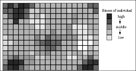
Fig. 8-3: Local model (diffusion evolutionary algorithm)

The local model (diffusion model) handles every individual separately and selects the mating partner in a local neighborhood by local selection, see Section 3.5. Thus, a diffusion of information through the population takes place. During the search virtual islands, see figure will evolve.
8.3 Regional model - Migration |
The regional model (migration model) divides the population into multiple subpopulations. These subpopulations evolve independently of each other for a certain number of generations (isolation time). After the isolation time a number of individuals is distributed between the subpopulation (migration). The number of exchanged individuals (migration rate), the selection method of the individuals for migration and the scheme of migration determines how much genetic diversity can occur in the subpopulation and the exchange of information between subpopulation.
The parallel implementation of the regional model showed not only a speed up in computation time, but it also needed less objective function evaluations when compared to a single population algorithm. So, even for a single processor computer, implementing the parallel algorithm in a serial manner (pseudo-parallel) delivers better results (the algorithm finds the global optimum more often or with less function evaluations).
The selection of the individuals for migration can take place:
Many possibilities exist for the structure of the migration of individuals between subpopulation. For example, migration may take place:
Fig. 8-4: Unrestricted migration topology (Complete net topology)
The most general migration strategy is that of unrestricted migration (complete net topology). Here, individuals may migrate from any subpopulation to another. For each subpopulation, a pool of potential immigrants is constructed from the other subpopulation. The individual migrants are then uniformly at random determined from this pool.
Figure gives a detailed description of the unrestricted migration scheme for 4 subpopulations with fitness-based selection. Subpopulation 2, 3 and 4 construct a pool of their best individuals (fitness-based migration). 1 individual is uniformly at random chosen from this pool and replaces the worst individual in subpopulation 1. This cycle is performed for every subpopulation. Thus, it is ensured that no subpopulation will receive individuals from itself.
Fig. 8-5: Scheme for migration of individuals between subpopulation
The most basic migration scheme is the ring topology. Here, individuals are transferred between directionally adjacent subpopulations. For example, individuals from subpopulation 6 migrate only to subpopulation 1 and individuals from subpopulation 1 only migrate to subpopulation 2.
Fig. 8-6: Ring migration topology; left: distance 1, right: distance 1 and 2
A similar strategy to the ring topology is the neighbourhood migration of figure . Like the ring topology, migration is made only between the nearest neighbours. However, migration may occur in either direction between subpopulations. For each subpopulation, the possible immigrants are determined, according to the desired selection method, from the adjacent subpopulations and a final selection is made from this pool of individuals (similar to figure ).
Fig. 8-7: Neighbourhood migration topology (2-D grid)
Figure shows a possible scheme for a 2-D implementation of the neighbourhood topology. Sometimes this structure is called a torus.
With the multipopulation evolutionary algorithm better results were obtained for many functions tested than for a single population algorithm with the same number of individuals. Similar results are reported in [Loh91], [MSB91], [Rud91], [SWM91], [Tan89], [VBS91], [VSB92] and [Can95].
| GEATbx: | Main page Tutorial Algorithms M-functions Parameter/Options Example functions www.geatbx.com |