

| GEATbx: | Main page Tutorial Algorithms M-functions Parameter/Options Example functions www.geatbx.com |
Evolutionary algorithms are stochastic search methods that mimic the metaphor of natural biological evolution. Evolutionary algorithms operate on a population of potential solutions applying the principle of survival of the fittest to produce better and better approximations to a solution. At each generation, a new set of approximations is created by the process of selecting individuals according to their level of fitness in the problem domain an d breeding them together using operators borrowed from natural genetics. This process leads to the evolution of populations of individuals that are better suited to their environment than the individuals that they were created from, just as in natural adaptation.
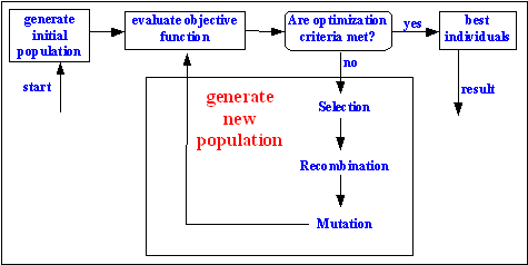
Evolutionary algorithms model natural processes, such as selection, recombination, mutation, migration, locality and neighborhood. Figure shows the structure of a simple evolutionary algorithm. Evolutionary algorithms work on populations of individuals instead of single solutions. In this way the search is performed in a parallel manner.
Fig. 2-1: Structure of a single population evolutionary algorithm

At the beginning of the computation a number of individuals (the population) are randomly initialized. The objective function is then evaluated for these individuals. The first/initial generation is produced.
If the optimization criteria are not met the creation of a new generation starts. Individuals are selected according to their fitness for the production of offspring. Parents are recombined to produce offspring. All offspring will be mutated with a certain probability. The fitness of the offspring is then computed. The offspring are inserted into the population replacing the parents, producing a new generation. This cycle is performed until the optimization criteria are reached.
Such a single population evolutionary algorithm is powerful and performs well on a wide variety of problems. However, better results can be obtained by introducing multiple subpopulations. Every subpopulation evolves over a few generations isolated (like the single population evolutionary algorithm) before one or more individuals are exchanged between the subpopulation. The multi-population evolutionary algorithm models the evolution of a species in a way more similar to nature than the single population evolutionary algorithm. Figure shows the structure of such an extended multi-population evolutionary algorithm.
Fig. 2-2: Structure of an extended multipopulation evolutionary algorithm
From the above discussion, it can be seen that evolutionary algorithms differ substantially from more traditional search and optimization methods. The most significant differences are:
The following sections list some methods and operators of the main parts of Evolutionary Algorithms. A thorough explanation of the operators will be given in the following chapters.
2.1 Selection |
Selection determines, which individuals are chosen for mating (recombination) and how many offspring each selected individual produces. The first step is fitness assignment by:
The actual selection is performed in the next step. Parents are selected according to their fitness by means of one of the following algorithms:
For more info see Chapter 3.
2.2 Recombination |
Recombination produces new individuals in combining the information contained in the parents (parents - mating population). Depending on the representation of the variables of the individuals the following algorithms can be applied:
For the recombination of binary valued variables the name 'crossover' is established. This has mainly historical reasons. Genetic algorithms mostly used binary variables and the name 'crossover'. Both notions (recombination and crossover) are equivalent in the area of Evolutionary Algorithms. For consistency, throughout this study the notion 'recombination' will be used (except when referring to specially named methods or operators).
For more info see Chapter 4.
2.3 Mutation |
After recombination every offspring undergoes mutation. Offspring variables are mutated by small perturbations (size of the mutation step), with low probability. The representation of the variables determines the used algorithm. Two operators are explained:
For more info see Chapter 5.
2.4 Reinsertion |
After producing offspring they must be inserted into the population. This is especially important, if less offspring are produced than the size of the original population. Another case is, when not all offspring are to be used at each generation or if more offspring are generated than needed. By a reinsertion scheme is determined which individuals should be inserted into the new population and which individuals of the population will be replaced by offspring.
The used selection algorithm determines the reinsertion scheme:
For more info see Chapter 6.
2.5 Population models - parallel implementation of evolutionary algorithms |
The extended management of populations (population models) allows the definition of extensions of Evolutionary Algorithms. These extensions can contribute to an increased performance of Evolutionary Algorithms.
The following extensions can be distinguished:
For more info see Chapter 8.
2.6 Application of multiple/different strategies and competition between subpopulations |
Based on the regional population model the application of multiple different strategies at the same time is possible. This is done by applying different operators and parameters for each subpopulation. For an efficient distribution of resources during an optimization competing subpopulations are used.
These extensions of the regional population model contribute to an increased performance of Evolutionary Algorithms, especially for large and complex real-world applications.
For more info see Chapter 9.
| GEATbx: | Main page Tutorial Algorithms M-functions Parameter/Options Example functions www.geatbx.com |